Much of my research focuses on the dynamic relationships between assets in the market (#1,#2,#3).  Typically, I use correlation as a measure of relationship dependence since its results are easy to communicate and understand (as opposed to mutual information, which is somewhat less used in finance than it is in information theory).  However, analyzing the dynamics of correlation require us to calculate a moving correlation (a.k.a. windowed, trailing, or rolling).

Moving averages are well-understood and easily calculated – they take into account one asset at a time and produce one value for each time period.  Moving correlations, unlike moving averages,  must take into account multiple assets and produce a matrix of values for each time period.  In the simplest case, we care about the correlation between two assets – for example, the S&P 500  (SPY) and the financial sector (XLF).  In this case, we need only pay attention to one value in the matrix.  However, if we were to add the energy sector (XLE), it becomes more difficult to efficiently calculate and represent these correlations.  This is always true for 3 or more different assets.

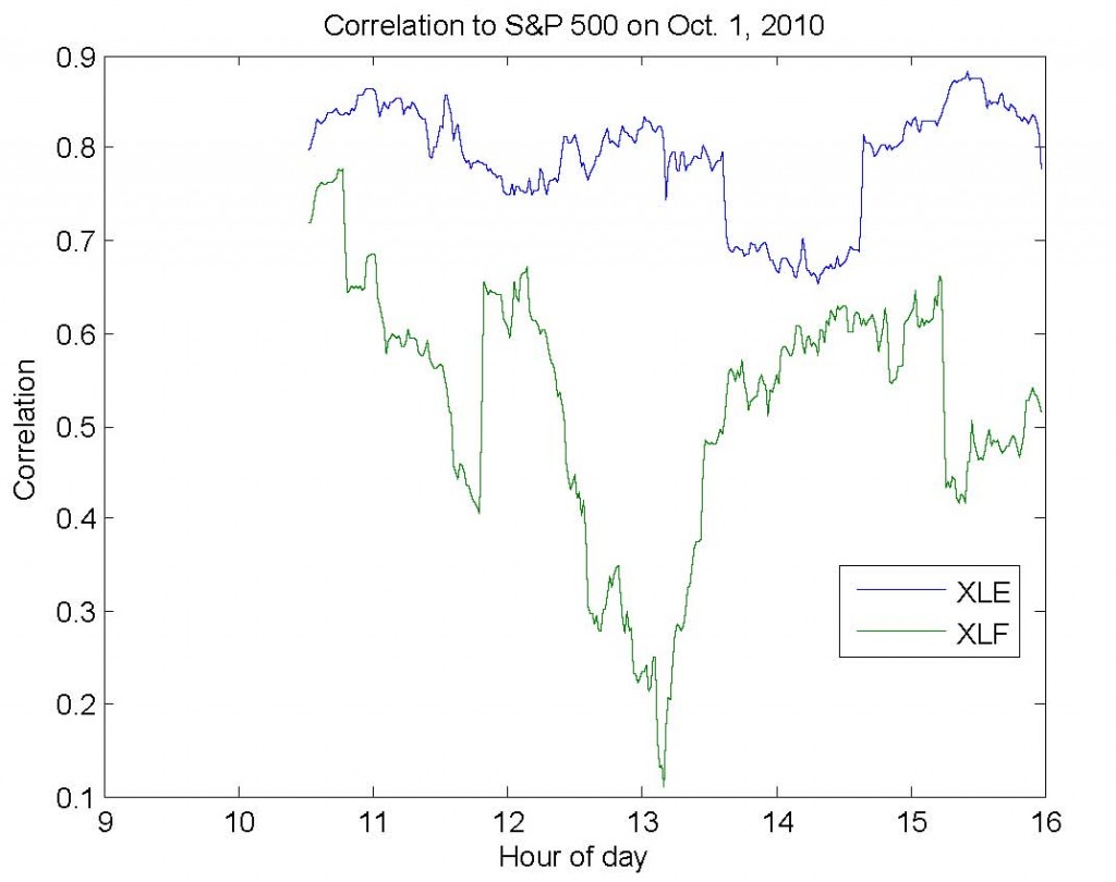
I’ve written the code below to simplify this process (download).  First, you provide a matrix (dataMatrix) with variables in the columns – for example, SPY in column 1, XLF in column 2, and XLE in column 3.  Second, you provide a window size (windowSize).  For example, if dataMatrix contained minutely returns, then a window size of 60 would produce trailing hourly correlation estimates.  Third, you indicate which column (indexColumn) you care about seeing the results for.  In our example, we would likely specify column 1, since this would allow us to observe the correlation between (1) the S&P and financial sector and (2) the S&P and energy sector.

The image below shows the results for exactly the example above for last Friday, October 1st, 2010.
This post was originally published on April 13th, 2008.  It was imported from a previous version of the site.

I normally don’t delve too much into the programmatic details of my work, but I’ve seen enough interest in this topic that I figured I’d lend a helping hand to those fellow frustrated souls.

There are a few awkward, non-native MEX implementations of various database interfaces.  However, Matlab has its own database toolbox built around ODBC/JDBC, and when developing distributable software, one always hopes to minimize third-party library usage.  As a result, I’ve put a good deal of effort into integrating Matlab with both MySQL and SQLite.  In fact, the data for every post on this site is stored in a 2GB MySQL database server running on my laptop.

As you can see, this requires only that you distribute the platform-independent JAR.  No DLLs, no MEX compilation.

% Database Server
host = 'localhost';

% Database Username/Password
user = 'user'; password = 'password';
% Database Name
dbName = 'assets'; 
% JDBC Parameters jdbcString = sprintf('jdbc:mysql://%s/%s', host, dbName); jdbcDriver = 'com.mysql.jdbc.Driver';
% Set this to the path to your MySQL Connector/J JAR
javaaddpath('mysql-connector-java-5.1.6-bin.jar')
% Create the database connection object dbConn = database(dbName, user , password, jdbcDriver, jdbcString);
% Check to make sure that we successfully connected if isconnection(dbConn)     % Fetch the symbol, market cap, and last close for the 10 largest % market cap ETFs     result = get(fetch(exec(dbConn, 'SELECT info.symbol,info.marketcap,series.close FROM info, series WHERE info.type=''ETF'' AND info.id = series.symbolid AND series.date = ''2008-04-11'' ORDER BY marketcap DESC LIMIT 10')), 'Data');     disp(result);
% If the connection failed, print the error message else     disp(sprintf('Connection failed: %s', dbConn.Message)); end % Close the connection so we don't run out of MySQL threads close(dbConn);
Output:
    ‘SPY’     [8.2300e+010]    [133.3800]
    ‘EFA’     [4.5420e+010]    [ 72.6400]
    ‘EEM’     [2.3850e+010]    [139.3400]
    ‘GLD’     [1.9260e+010]    [ 91.3000]
    ‘QQQQ’    [1.7040e+010]    [ 44.2800]
    ‘IVV’     [1.6410e+010]    [133.5200]
    ‘IWF’     [1.2860e+010]    [ 55.2500]
    ‘DIA’     [1.0830e+010]    [123.3400]
    ‘IWM’     [1.0470e+010]    [ 68.7200]
    ‘VTI’     [9.7800e+009]    [132.2900]

This post was originally published on September 3rd, 2007. It has been slightly modified from a previous version of the site.  N.B.: This code has been tested in Matlab R2009b and R2010a and still works fine.

Kaplan and Knowles, extending the original work of Shadwick and Keating as well as that of Kazemi, Schneeweis, and Gupta, describe a generalized downside risk-adjusted measure Kappa.  By design, the Omega and Sortino measures are special cases of the Kappa measure, and, as such, the Kappa function is capable of calculating both easily.

So that this very helpful function can be used by those in the community who are having difficulty with the original works, I am publishing a single-line Kappa function for Matlab.

% D : return series vector
% r : return threshold
% n : Kappa order
function k = kappa(D, r, n)
k = (mean(D) - r) ./ nthroot(mean((D < r) .* (r-D).^n), n);

To calculate the Omega measure, put n=1 and add 1 to the result, i.e. kappa(D, r, 1) + 1.

To calculate the Sortino ratio, put n=2, i.e. kappa(D,r,2).