Last week, I posted a zoomable visualization of the weekly market and sector performance and correlation.  People seem to find this image both useful and “cool,” so here is this week’s edition and takeaways below:

  • Green, green, green (on the diagonal).  Other than healthcare  (XLV), every sector was up at least 1%, and most were up well over 3%.
  • More green (off the diagonal).  Most sectors were strongly correlated with one another, with the exception of financials (XLF) and healthcare (XLV).  Healthcare, as noted above, underperformed the market significantly by 2.5%.  The story with financials is the opposite – financials were up a whopping 6.8% this week, putting them over 3% ahead of the market.
  • Correlation was strongest between energy (XLE) and materials (XLB) at 99.5% and weakest between financials (XLF) and healthcare (XLV) at -21.8%.


By the way, this figure is produced with Python and cairo.  The code is fairly ugly and long, so I probably won’t release it unless there’s some demand.

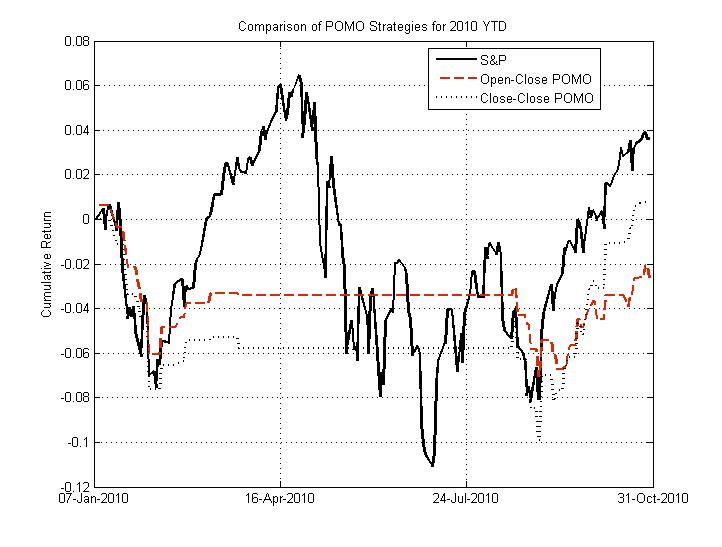
Since I’m sick of hearing ZeroHege purposefully misstating the empirical relationship between POMO and the equity market, I decided to put up this little figure below. This figure demonstrates the performance of the S&P 500 (SPY) in solid black compared to two POMO strategies in dashed black and red (close-close and open-close, respectively).

Note that only holding the market on POMO days has not returned more than the buy-and-hold S&P 500 strategy year-to-date. The S&P 500 has returned 3.62% YTD (close-close, not including dividend, which puts the buy-hold strategy even further ahead), whereas the open-close and close-close strategies have returned -2.63 and 0.79% respectively. These strategies do not even outperform the S&P 500 on a risk-adjusted basis (Sharpe). Furthermore, none of the regressions that were significant (p=0.05) in the 2005-2010 dataset are significant (p=0.1) in the 10 months through this year. In other words, though a relationship between the accepted-submitted proportion and return magnitude exists in the dataset as a whole, this relationship appears to have disappeared on the daily timescale.  Sorry, Tyler(s).

What would happen if you took the Index and Sector Summary Heatmap I made last week, blew it up to the size of a 36MP image (6000-by-6000), and then added a plot of the change in correlation over time. Great question! Look below.

Since there’s a lot going on here, let’s summarize what’s going on:

  • Make sure you zoom into the figure!  You can use the scroll wheel on your mouse or two-finger slide on your touchpad to quickly zoom in and out.
  • Each diagonal cell shows the return of each asset over the past week (6 periods, 5 returns). As an asset increases, the line is colored green, and as an asset decreases, the line is colored red.
  • The lower left hand corner of each diagonal cell  shows the total return of the asset over the past week.  There’s also a label down there, in case you’re zoomed in and can’t see the labels on the edge.
  • The off-diagonal cells show the correlation (5-period return) between two assets.  The color of the cell indicates the degree of correlation – more correlated assets are more green, and less correlated assets are more red.  In case you’re zoomed in, there’s a label in the lower left hand corner that tells you which two assets you’re looking at.
  • The off-diagonal cells also show the time series of 5-day return correlation over the past 4 weeks.

It seems like many of my posts lately have been critical of others lately (#1: POMO, #2: Dollar / Gold, #3: Twitter ).  On the downside, everybody wants to get along and nobody makes friends on the attack.  On the upside, it’s good for plenty of site hits and provides two sides to a discussion.

So what the hell, here it goes – here’s why I think the ZeroHedge submitted/accepted ratio post gets it wrong. (Note that all of the analysis, both here and by John Lohman, suffers from an in-sample issue.  None of this is really a strategy that could be implemented without information about the submitted-to-accepted ratio in advance.  This may still be profitable if you took the positions at 11am instead of 9:30am, but none of the data we’re providing proves it.  I will be performing real intraday analysis with out-of-sample backtesting in the  paper I’m working on right now).

First of all, I think John Lohman’s logic is mostly right in the hypothesis.  If the “conspiracy theory” is really true, then the ratio of submitted-to-accepted should be proportional to the market’s return.  However, there are a few points I’d like to make for rigor’s sake here.

  • First, why can’t PDs go short too?  Maybe it makes more sense to put the absolute value of the market’s return on the LHS, dropping the sign. (Hint: See below if you want the answer!)
  • Second, there are a number of alternate hypotheses that are not conspiracy-like that could also result in this proportional relationship.  Maybe market participants just take some days of the week off, and the Fed chose to schedule POMO on days that would have higher liquidity anyway.  If you were Brian Sack, wouldn’t you want to schedule these operations on days where the most PDs would participate or they would be best staffed?
  • Third, just to emphasize it again, neither John nor I are actually presenting these analyses as something you can take to the market.  The submitted-accepted ratio comes out after the operation begins, which is never before 9:30am, which means you could never realize the returns we’re showing precisely.  For a strategy you can actually execute, see yesterday’s post (but don’t assume it’s profitably stable).
  • Fourth, I’ve switched from submitted-to-accepted to accepted-to-submitted.  This makes everything easier to see and interpret.

OK, so again, John’s logic is decent enough.  If I had to guess, Tyler at ZH likely added his own emphasis to the post “for effect,” which might have masked some of John’s real tone.  So down to the brass tacks and the data.  First of all, I’m using the SPY for the S&P 500 and my POMO dataset for information on the submitted-to-accepted ratio.  I’m also publishing the Matlab code here, just for full disclosure sake.

Now, if you run this code, you’ll see the following two scatter plots pop up.  The red are the bottom third of the POMO operations by accepted-to-submitted ratio, the blue are the middle third, and the green are the top third.
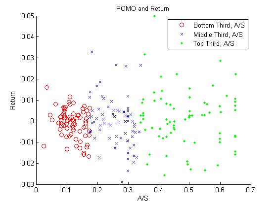
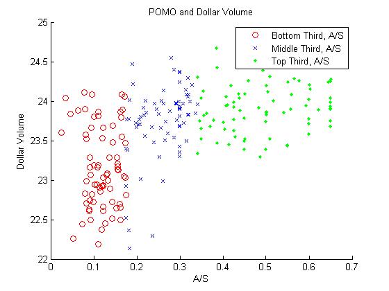
OK, so it looks like there’s definitely something going on for the dollar volume.  However, the story for the return is a little bit more fuzzy.  It appears that the spread increases as the accepted-to-submitted ratio increases, but not necessarily that there is a strong direction to the sign.  Maybe, as I mentioned above, the magnitude of the return is what’s  proportional, not just the value.  As you can see in the Matlab code, I fit a simple GLM for each of these and get the following:

  • log(close) – log(open) ~ accepted/submitted ratio: The coefficient on the ratio is slightly positive (0.0066, +-0.0047) but the t-stat is 1.4.  No go.
  • log(dollar volume) ~ accepted/submitted ratio: The coefficient is on the ratio is definitely positive (1.75, +-0.18) and the t-stat is 9.6.  This conclusion is definitely supported – the ratio of accepted-to-submitted is proportional to the total dollars traded on SPY.
  • abs(log(close) – log(open)) ~ accepted/submitted ratio: In this case, the coefficient is definitely positive (0.0159, +-0.0032) and the t-stat 5.0.  This conclusion is also supported – the ratio of accepted-to-submitted is proportional to the magnitude of SPY’s return, but not necessarily the direction.

So there you have it – the dollar volume and magnitude of the change are statistically significantly related to the POMO accepted-to-submitted ratio, but the direction is not really guaranteed.  Much more of this to come in a research paper I’m currently working on.
Heatmaps have been all the rage this week. I was driving down US-23 to Ann Arbor last Monday and heard Jim Cramer introduce the thing to Erin Burnett.  My first instinct was that we’d see something like this, followed by a rant from Mark Haines.  However, the real thing turned out to be much more tame and reasonable.

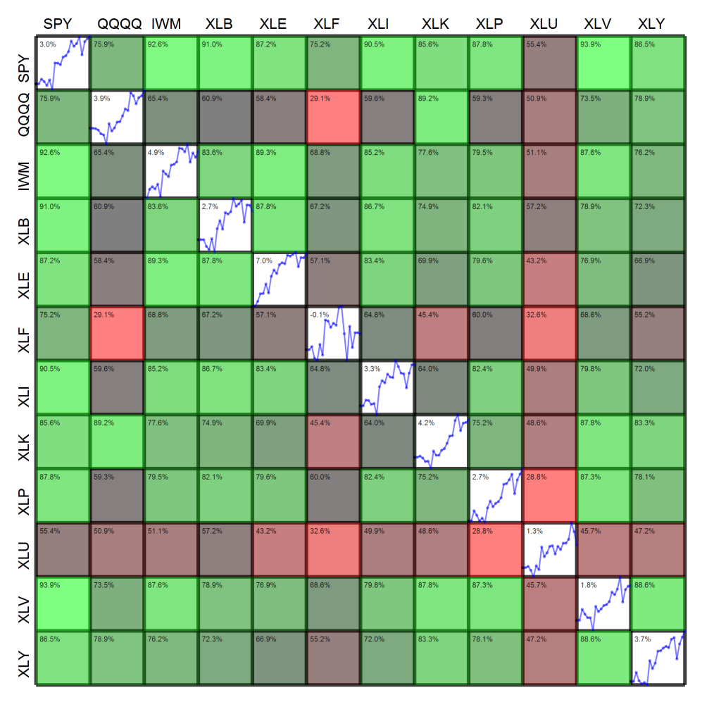
Now that heatmaps are en vogue, I figured I’d take my own shot at one.  I’ve always been a fan and use them in publications, but there’s a very fine line between conveying large amounts of information intuitively and just overloading the viewer.  The figure below shows two pieces of information simultaneously:

  1. The diagonal cells show the cumulative log-return time series of each asset over the past month.  The upper left hand corner of the diagonal cell displays the past month’s return.
  2. Off-diagonal cells show the color-coded correlation between assets.  For example, reading across the first row shows the correlation of each asset with the S&P 500.  Reading the figure indicates that the S&P 500 (SPY) has a correlation coefficient of 75.9% with the Nasdaq (QQQQ) and 92.6% with the Russell 2000 (IWM).  The upper left hand corner of these off-diagonal cells displays the correlation coefficient.

Please let me know what you think of the figure, pro or con.  If you’ve got any other suggestions, also feel free to leave a comment.  Note that there are a still a few “degrees of visualization freedom,” e.g., thickness of cell borders, opacity of cells, plenty of free pixels in the interior of cells.   For instance, how would you suggest I convey information about the volatility of each fund over the week?

This post was originally published on April 30th, 2007. It was imported from a previous version of the site.

Coming on the heels of my look at the overall ETF market in the last three months, and using the same data set, this entry is meant to provide an overview of the country-specific MSCI ETFs.

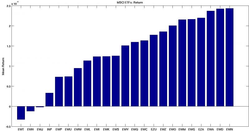
So the average MSCI ETF gained about 0.14% daily, with the Netherlands in first and Taiwan in last.  The trend is relatively clear – most economies have seen solid growth, while Taiwan, Hong Kong, and Japan have struggled to tread water.  It’s interesting to note that the same issues do not seem to have affected Singapore, Malaysia, or Korea.

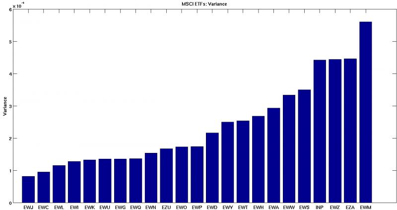
As far as volatility goes, Malaysia clearly leads the pack, with South Africa, Brazil, and India close behind.  On the other end, all seems quiet for Japan and Canada, as well as most of the European economies.

Overall, it looks like as far as the MSCI is concerned, Europe gives higher yield with less risk compared to any of the BRICS acronym variants (Brazil, India, S. Africa, Mexico, etc.).  Whether this trend will continue is another question, especially given the recent rise of lending rates, but it’s hard not to price in the relative stability of western European countries like the Netherlands when compared to Malaysia.