This post was originally published on April 13th, 2008. It was imported from a previous version of the site.
The simple moving average is easily the most fundamental indicator in technical analysis, and though there are many ways to use it, Tom Lydon of ETF Trends gives an example here. I wanted to go into some detail on the relationship between the moving average and its predictive power, as I’ve done some comprehensive analysis of similar strategies in the currency markets. Following along with Tom, I’ve decided to use the SPY tracker ETF for this example.
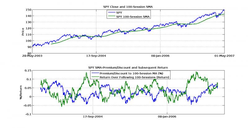
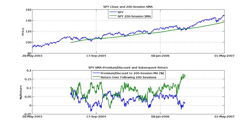
What I’ve done here is something similar to premium/discount analysis. Pretend that the moving average is some underlying valuation, and look at what percentage above or below that price the ETF is actually trading. You can see the actual close price and the moving average calculated on it in the top panel. In the bottom panel, you’ll see the percentage of premium discount (in decimal form, e.g. 0.05 = 5%), as well as the cumulative return over the next N sessions.
To give some comparable horizon, I fixed the return outlook to the exact length of the moving average. That is, if the premium/discount is calculated over the moving average of the last 100 sessions, I look at the return over the next 100 days. Though this fails to take into account stop-loss strategies or other trailing/bracketed order methods, it gives a better picture of how the premium/discount factor and the actual market are correlated. Furthermore, though discipline in your loss minimization is an absolute must, it makes much more sense to invest when the trend is more in your favor, both for actual performance and tax purposes.
So here are these calculations for both 100- and 200-sessions. Note that the bottom panel of each graph only shows regions over which the numbers make sense, that is, once the moving average can be calculated and while there is still a full return period remaining.


For both graphs, the results look surprisingly symmetric. When the premium is high, returns are low, and if the SPY is actually trading at a discount to its moving average, buy-buy-buy! Accumulating when at or below the moving average seems to be a much better strategy for longer term holds. For example, on the 200-session moving average, buying blocks when the SPY traded near par and selling them dumbly after 200 days, you’d make a little over 10% on average. Following a similar strategy for the 100-session and buying blocks at about 3% discount yields even higher average returns!
There are a few important things to note though. First, this does not beat a vanilla buy-and-hold forever strategy for return, but it does reduce the value at risk. For most portfolios, one trumps the other! Secondly, this strategy is only shown here when the derivative of the 200-session moving average is positive, that is, when the 200-session trend line is increasing. This strategy is much more profitable when the 200-session moving average is not downward sloping, and I think this is where Tom’s wisdom comes from. Though you might miss the initial rally that leads the moving average into a positive trend, you also miss all the times it doesn’t.
Though you can’t backtest the future, and index trackers are far different beasts than specialized ETFs, this data seems to point to a dumb yet successful strategy similar to premium strategies that bond and mutual fund traders often employ. Though no replacement for disciplined loss management, it does seem to warrant further attention across the broader range of ETF products.


